Object Detection with Create ML: training and demo app
You’ve collected images, annotated them for object detection, and exported your dataset. Gazing in wonder at Xcode, the thought creeps in… what now? Answer: we’ll import the data into Create ML, configure training parameters, perform training itself, reckon with our results, and integrate the model into a demo application. Along the way, we’ll offer some insights about some of the algorithms and frameworks that make this futuristic sorcery come to life. Keep those eyes locked on the screen and start scrolling down!
Other parts:
- Object Detection with Create ML: images and dataset
- Object Detection with Create ML: training and demo app
This is the second part of a series introducing the fundamentals of working with Apple’s native ML tools. The goal here is to build an app that will be able to detect and highlight the appearance of a license plate in a video. (For instance, a video showing the front of a parked car should draw a box around the plate.) In the previous installment, we collected images from scratch, and prepared a dataset to work with Create ML. If you want to check out how we did it, or find out what parameters your data should adhere to—check out part 1 of our object detection guide!
Importing data to Create ML
Since we’ve got our three folders prepared, let’s jump right in and start working with Create ML. There are two ways to open the application. We can input “Create ML” in Spotlight Search or open Xcode and select Xcode → Open Developer Tool → Create ML from the drop-down menu.
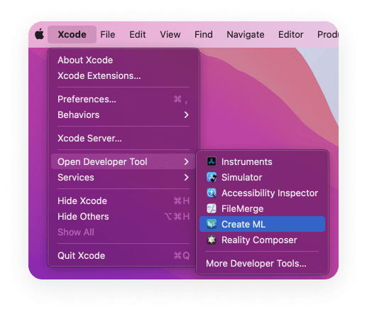
There it is… Create ML. You’re standing on the threshold of greatness here.
A file browser window will open, you’ll need to select New Document, then, once the app is open, we’ll create a new project. Select the Object Detection template, and let’s enter the project’s name (and any other info as you’d like in this field), then choose where the project will live on your machine, and continue onward. On the next screen, we’ll add our data to the appropriate fields. To add pre-trained images to the project, drag the corresponding folder into the required field:
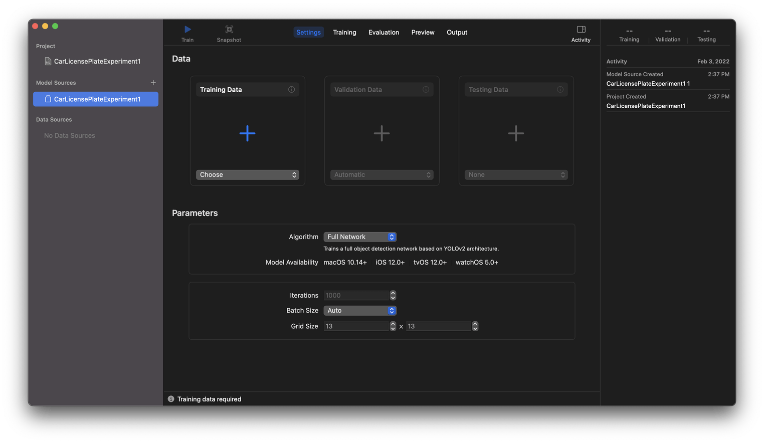
🤔 Three places to add data… and we have three folders of data.
Your Data section should now look something like this:
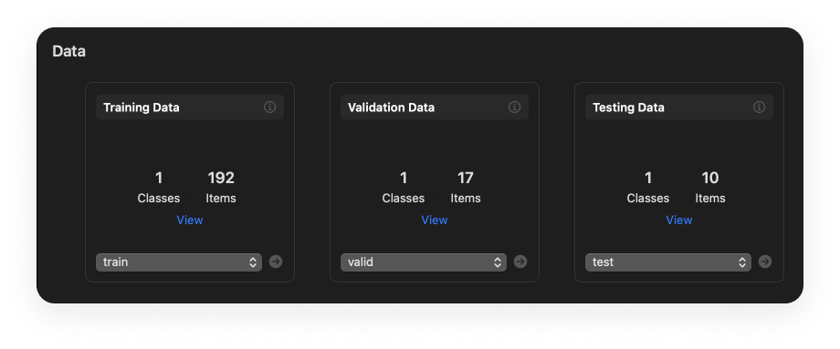
If you’re using your own dataset, expect the numbers to look different.
Training parameters
By default, Create ML prompts us to train our model using the YOLO algorithm. YOLO is one of the most effective algorithms for training Object Detection models. In Create ML, this is called full network.
The Iterations and Batch Size parameters are closely related to the concept of gradient descent—this is an algorithm for iterative optimization of neural network weights.
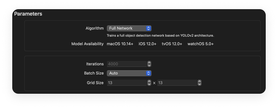
Loading all the data at once can be inefficient, and problems can often arise as a result. To help prevent this, the dataset is divided into smaller packets (this is called a batch) and is then processed by the algorithm on an iterative basis. During each iteration, a batch of a certain size (specified by the Batch Size parameter) is collected. Then, based on this batch, the algorithm makes predictions (it attempts to find the object in each of the batch’s images) and saves the results for further neural network corrections. At the end of each iteration, the model “calibrates” (that is, the weights are updated). Accordingly, the Iterations parameter describes the total number of iterations. So, an iterative gradient descent approach helps the model optimally adjust to the data.
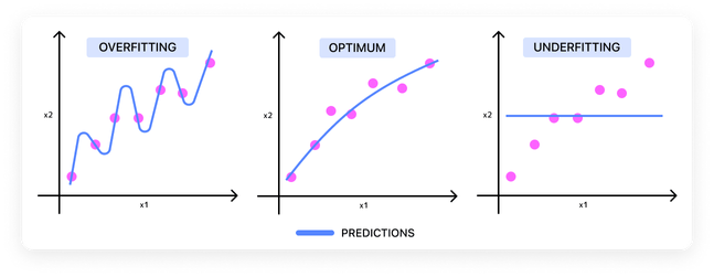
But a larger number of iterations do not always positively affect the model’s efficiency and can instead lead to overfitting. An overfit model won’t be able to recognize the desired data (in our case, license plates) in any image that wasn’t included in the training set. Or vice versa, if you take too few iterations, you’ll end up with underfitting, and the model will have a high chance of error.
Batch Size is equally important as the number of iterations. If Batch Size = 1, the model weights will be adjusted too often. And on the other side of things, it will happen once if Batch Size = dataset size.
Which parameters should we choose?
So, which parameter values should you choose?
Let’s start with Iterations. Based on my own experiments to determine this, it turns out that 1000-1500 iterations are enough for our purposes.
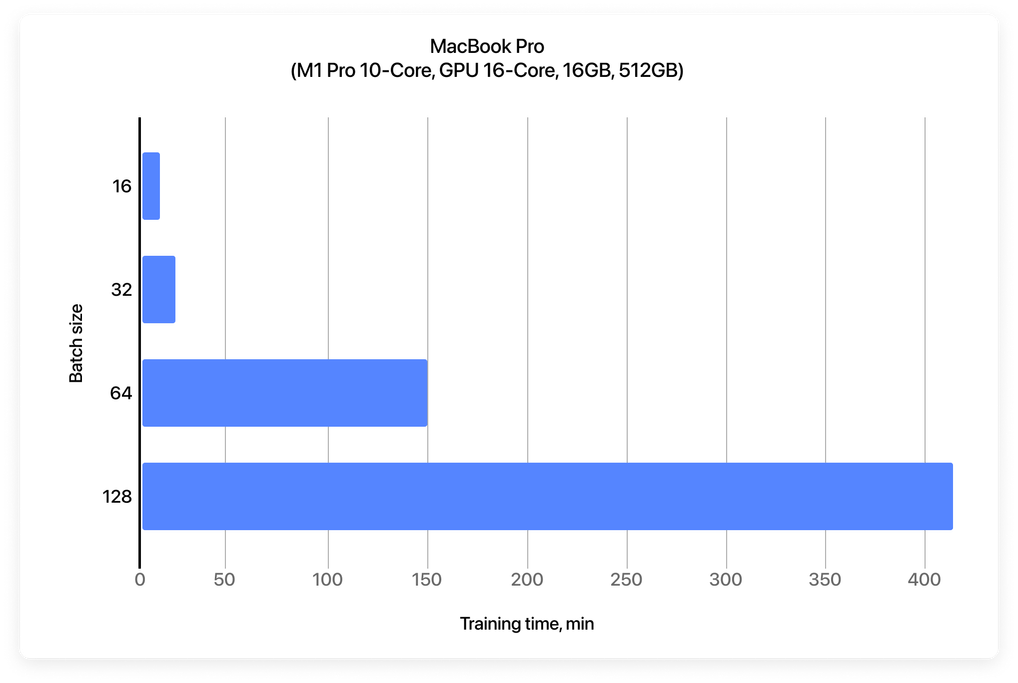
In one of its reports, Apple claims that the higher the batch size, the better. Still, the drop-down list offers several options: 16, 32, 64, 128, and Auto. When Auto is selected, the system chooses the batch size based on the performance of the current computer. (After trying all the options separately, we managed to find out that for a MacBook Pro with an M1 Pro chip Auto = 32.) The accuracy and efficiency of models trained with different values for Batch Size differ insignificantly because the size of our dataset is small, so to maximize model performance, minimize training time, and simplify our task, we’ll leave the value set to Auto.
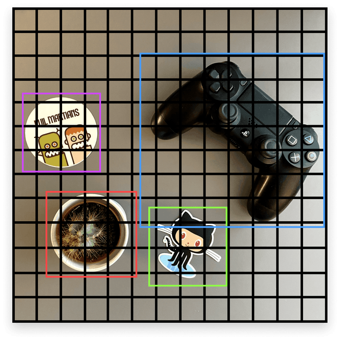
Moving on to the final parameter, Grid Size is the original image’s fragment grid with an S×S size; the algorithm automatically delineates this grid during processing. This is the main difference between the YOLO algorithm and other such algorithms. The grid size is determined based on the size of the object inside the image.
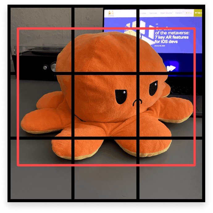
To explain this a bit more, to find an object that occupies 50-60% of the entire image, a 13×13 grid is likely to be overkill. In our set, all copies are square. Therefore, we will leave the value set to 13×13.
When you’re ready, click Train and let Create ML do its thing.
Analyzing our results
After training is finished, you can also run an additional number of iterations (by clicking Train More). In theory, this will increase accuracy, but it won’t have a significant difference. To more effectively increase our accuracy, we should change the initial data set. This can be done by copying the current set in the left panel, changing or expanding the dataset, and then start training from the beginning.
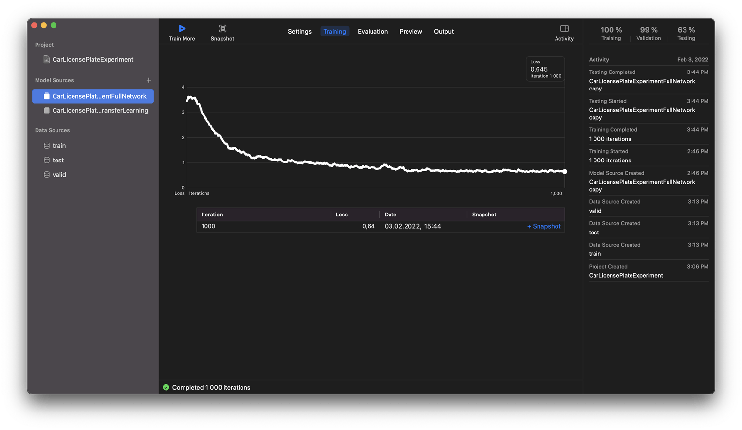
During training, Create ML builds a graph that displays values of the Loss function, which you can check out in the Training tab. The lower the value, the less mistakes the model makes. The picture below displays the results of using the full network (YOLO) algorithm. You can see the accuracy gradually increased until training was completed. I think that when the value of the Loss function is equal to 0.64, that indicates a pretty good result!
By selecting the Evaluation tab, you can see the metrics for the training, validation, and testing stages. For example, if our model included additional object classes besides car license plates, this table would display each class’s accuracy values. It’s handy for understanding which class prevails regarding the count of instances.
The I/U (intersection-over-union) value is a percentage from 0–100 which represents the overlap between the annotated box (this is included in the annotation JSON file) and the box which the model predicts. So, I/U 10% means they just barely overlap, which 95% I/U means they are a really close match.
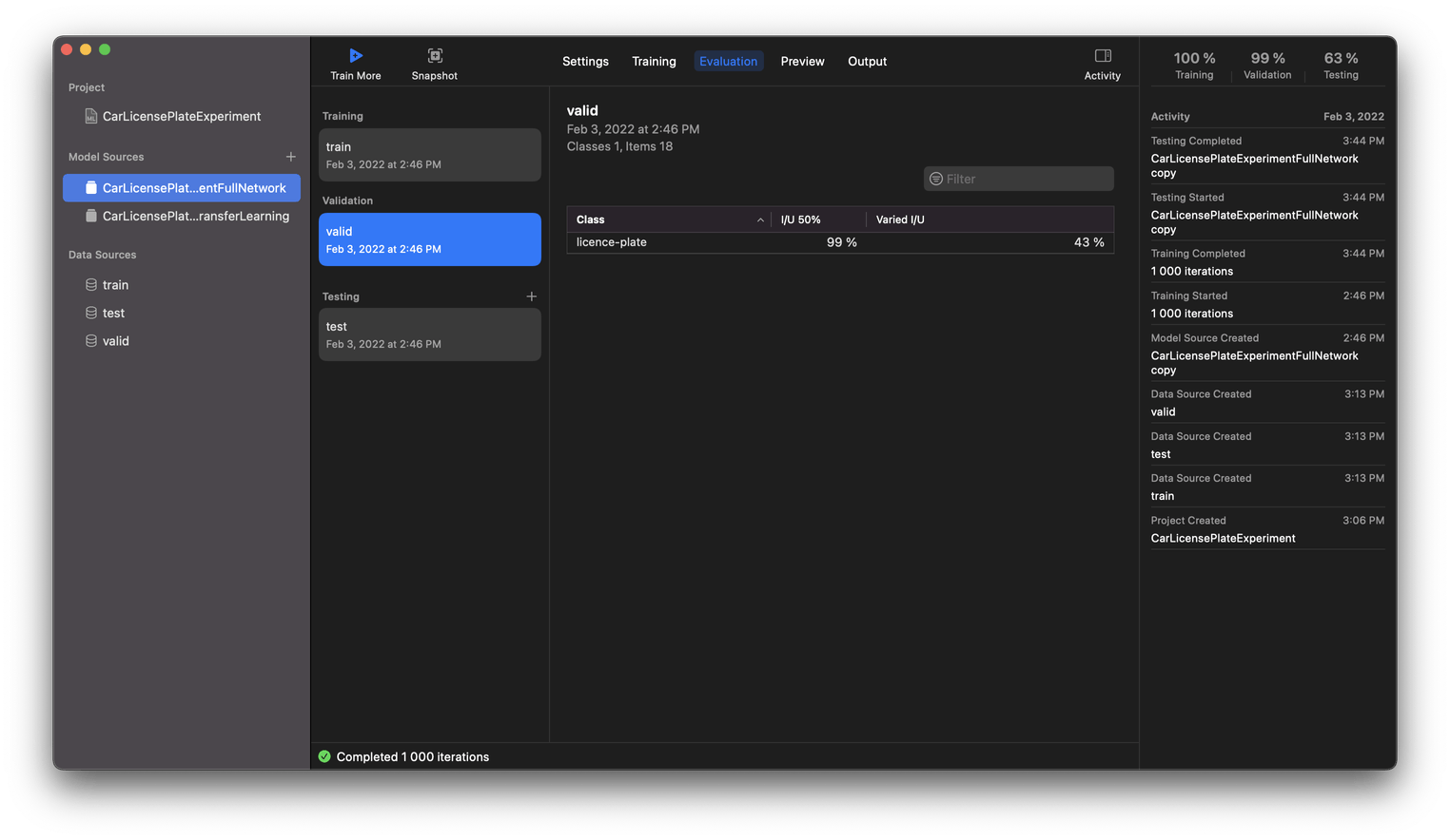
The percentages represent the average accuracy of predictions for each model class, and they are being calculated at two thresholds I/U 50% and Varied I/U. There aren’t a lot of resources online explaining what these thresholds mean (even from Apple), so let’s describe them a bit. I/U 50% is the value that indicates how many predictions have an accuracy higher than 50%. Varied I/U is the average value of prediction accuracy for a specific class in the dataset.
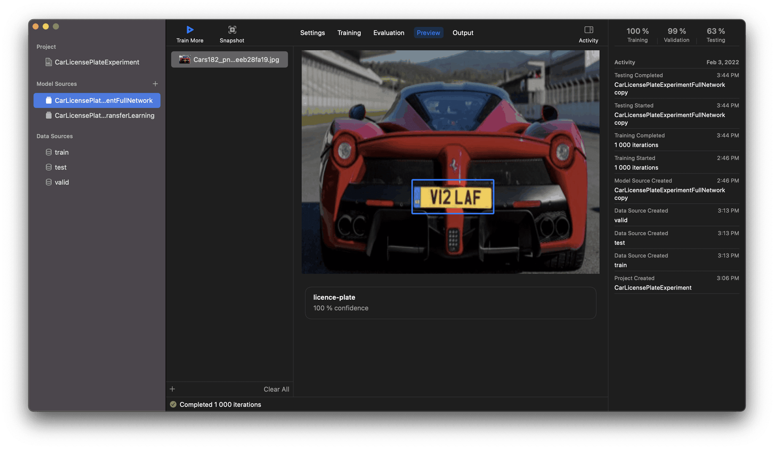
In the Preview tab, you can visually test the learning stage’s results. Simply drag images to the left list, and Create ML will show you the prediction as a blue box indicating the location of a license plate:
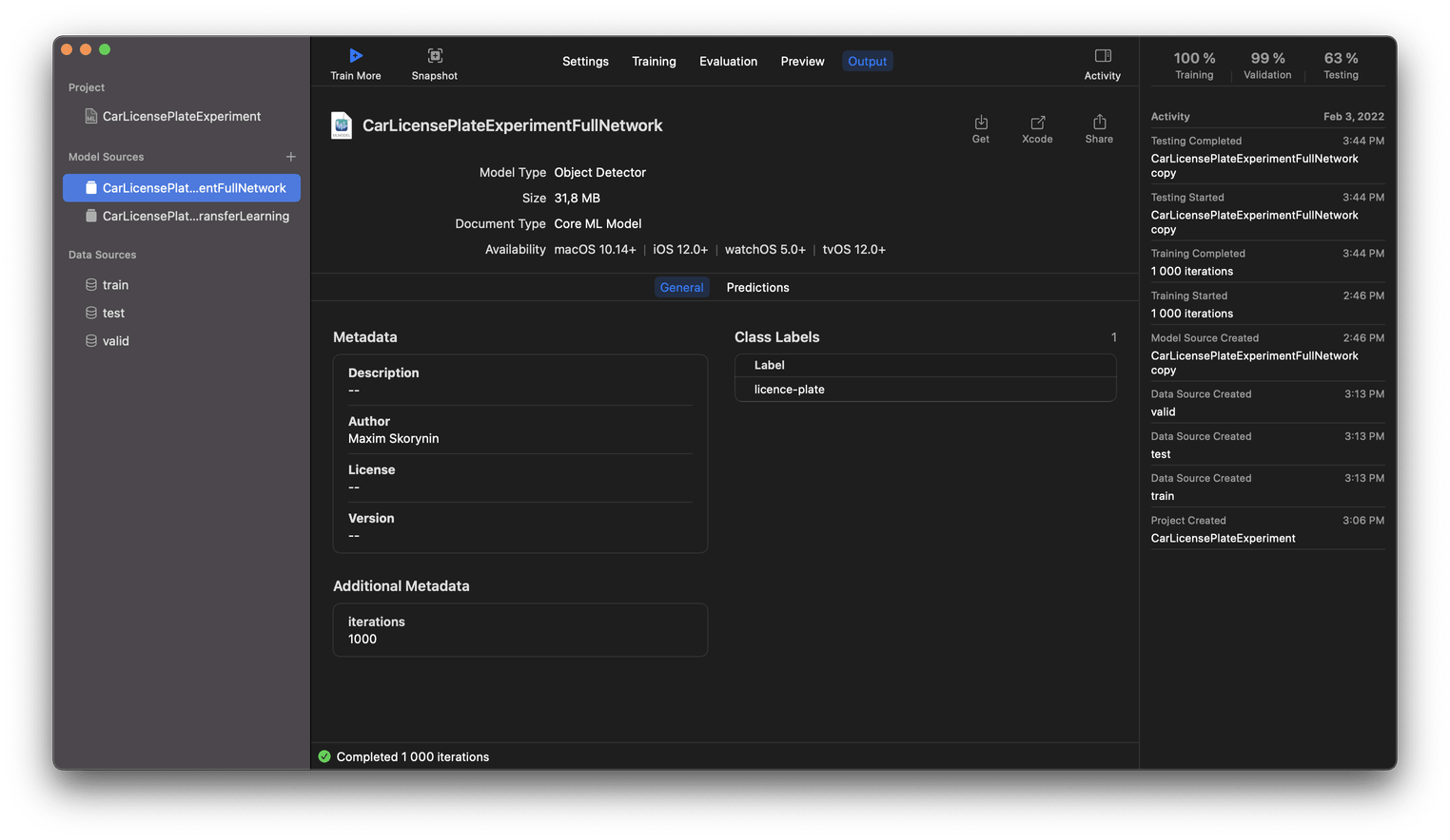
In the Output section, you can view model information, metadata and export your model.
Transfer Learning
Before moving on to app integration, let’s take a minute to touch on Transfer Learning, then we’ll compare results based on the chosen approach and hardware.
Transfer Learning entails building a new model based on one that’s already been trained. To make things clear, try and imagine that the existing model is sort of “transferring” its knowledge to the new model. And indeed, Apple provides such a model: it’s been trained on tons of images and is now being used as the foundation in Create ML. This approach allows for quicker results and the final file of the model is smaller in the end. By experiments. In order to get more accuracy with the Transfer Learning algorithm, we’ll need to prepare more initial data for training.
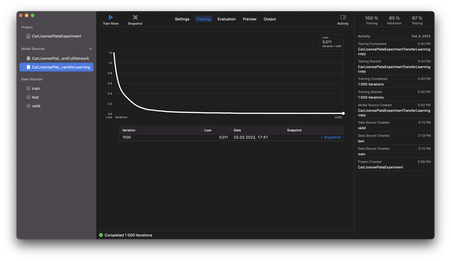
In the image below, you can see the model as trained by the Transfer Learning algorithm. It reached its loss function minimum value at about 250 iterations. This is because the size of the original set was small for this method. Still the speed is obviously faster, and the size of the final model is smaller.
Comparing training results
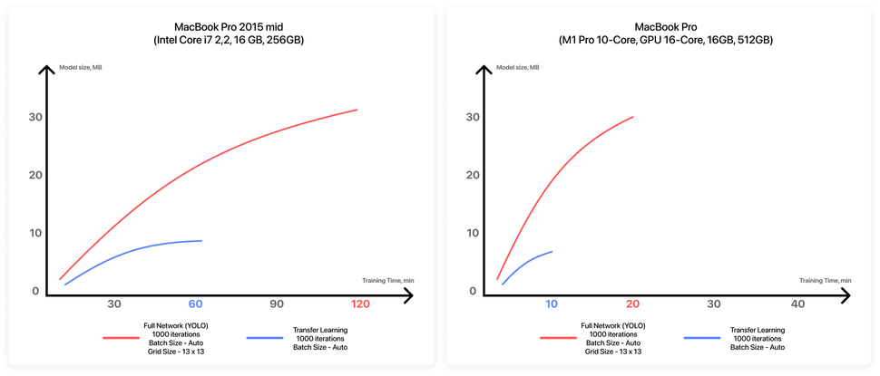
Let’s compare training performance and results based on device and chosen method (using a model created on Roboflow):
About the Vision framework
To integrate our model into a project, we’ll use the Vision framework. It’s available in Xcode for iOS 11.0+, and allows using a model as a class instance.
Vision works with models where video streams or image frames are being analyzed, for instance: Object Detection, Classification, Text Recognition, Action Classification, Hand Pose Classification.
Integrating our model into an iOS project
First, you should create a new iOS project and add the previously imported model to the root directory.
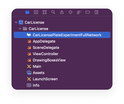
Since we’ll be using the camera, don’t forget to include the required attribute (Privacy - Camera Usage Description) in Info.plist.

Let’s walk through the main methods of setting up a model and processing a video stream.
In the setupRequest method, an object of the VNCoreMLRequest class is configured, taking two arguments as input: a model instance and a closure. The result will be passed to the closure. It is very convenient that after adding the model file to the project, we can use it as the CarLicensePlateExperimentFullNetwork class without additional effort.
private func setupRequest() {
    let configuration = MLModelConfiguration()

    guard let model = try? CarLicensePlateExperimentFullNetwork(configuration: configuration).model, let visionModel = try? VNCoreMLModel(for: model) else {
        return
    }

    request = VNCoreMLRequest(model: visionModel, completionHandler: visionRequestDidComplete)
    request?.imageCropAndScaleOption = .centerCrop
}
Now here’s the most important point to note: we’ll need to override the Sample Buffer Delegate for the camera’s output stream. Specifically, the captureOutput method which converts the video stream to the desired format and passes it on to the VNImageRequestHandler class object, that will launch the previously created request.
// MARK: - Video Delegate

extension ViewController: AVCaptureVideoDataOutputSampleBufferDelegate {

    func captureOutput(_ output: AVCaptureOutput, didOutput sampleBuffer: CMSampleBuffer, from connection: AVCaptureConnection) {
        guard let pixelBuffer = CMSampleBufferGetImageBuffer(sampleBuffer), let request = request else {
            return
        }

        let handler = VNImageRequestHandler(cvPixelBuffer: pixelBuffer)
        try? handler.perform([request])
    }

}
Pay attention to the code below as well—don’t forget to set self as a delegate of the output object.
private func setupCaptureSession() {
    ...
    let queue = DispatchQueue(label: "videoQueue", qos: .userInteractive)

    let output = AVCaptureVideoDataOutput()
    output.setSampleBufferDelegate(self, queue: queue)
    ...
}
The result will be passed to the visionRequestDidComplete method as an instance of the VNRequest class. We’ll then get the VNRecognizedObjectObservation array using the VNRequest object. VNRecognizedObjectObservation is an object which contains prediction results and some parameters:
labels: [VNClassificationObservation]: an object classifierboundingBox: CGRect: the size and location of an objectconfidence: [Float]: prediction accuracy from 0 to 1
Using the values of the boundingBox parameter, we can draw the frame on the screen. You can see a sample rendering in the demo project repository.
private func visionRequestDidComplete(request: VNRequest, error: Error?) {
    if let prediction = (request.results as? [VNRecognizedObjectObservation])?.first {
        DispatchQueue.main.async {
            self.drawingBoxesView?.drawBox(with: [prediction])
        }
    }
}
Result accuracy
Let’s compare the accuracy of our results using the full network algorithm versus Transfer Learning:

Preview tab results
And here it is in action inside the iOS app:
Conclusion detected
So, let’s summarize what we’ve done across the series. Despite a relatively small dataset, we managed to achieve a fairly good result! (Additionally, I’d like to note the performance of the new MacBook Pro with new generation M1 chips, which can increase model learning time up to 6 times.)
Core ML and Create ML are very powerful tools with many possibilities. I’m delighted that Apple is advancing machine learning and is constantly improving its tools. However, at present, detailed documentation is not really available, just a few small articles from Apple. So, when you want to go deeper into this topic or better understand the nuances of the configurable parameters inside Create ML, you have to collect information on the Internet, literally, bit by bit. This can really slow down the learning process. Hopefully this article opens that up a bit.
I’ve tried to share here what I thought was missing when I first started working with ML. I hope I was able to tell you something new and you now have more confidence and knowledge about the process of marking up a dataset and creating an Object Detection model from scratch. Once you know what you’re doing, the process is quite simple! And this is great because it means experiments and demos are fairly easy to get off the ground.
By the way, if you’ve got a problem, (ML-related or not) Evil Martians are ready to help! We’ll detect it, analyze it, and to zap it out of existence! (Or, if you’re missing something, we’ll zap it in to existense!) Drop us a line!

